Tutorial

Introduction

Designing nano-optical devices is a huge and complex task. A lot of steps have to be performed just right. Starting from the initial design to fabrication and testing. This software library is designed to make your life easier in one regard: The actual design of the chip.

In this tutorial we will create:

• A simple chip: First create a simple loop
• Simple Drawing: A gentle introduction on how to generate polygons and do boolean operations.

Software design and intended usage

Let’s first talk about some fundamental library design choices. If you are new, you might not understand everything. That’s OK, though. Head back here once you got the hang of it.

Under normal circumstances all geometric shapes and operations should be generated in Shapely. This will already give you a full repertoire of powerful geometric operations. These objects can then be converted to gdsCAD geometric objects. Since those already represent the polygons which will end in the final GDSII file it also follows the serious restrictions of the GDSII file format. Those restrictions will already be respected when converting the Shapely object. The conversion function is called gdshelpers.geometry.convert_to_gdscad().

While it looks like you’d need to call get_shapely_object() every time you want to convert it to gdsCAD by convert_to_gdscad(), you actually do not. If an object passed to convert_to_gdscad() has the get_shapely_object() method, it will be called for you and the resulting Shapely object will be converted instead. Note, that Shapely objects do not know layers, GDSII datatypes etc. You can specify those when converting to gdsCAD.

A simple chip

Creating the project

In PyCharm, create a new project called gds_tutorial at a location of your choice. Make sure you select the virtual environment interpreter which you set up in the install guide.

Add a new python file via New->New->Python file, called chip.py. An editor opens with a nearly empty file, you may ignore the __author__ line and delete it at will.

Hello World

To test that everything is working, let’s just put a print "Hello World" in chip.py. Of course this will just print Hello World on the console. Right click on chip.py and select Run `chip`.

Your program is directly executed and you can see the result on the bottom of the screen in the terminal.

This action has create a run profile for this file. If you create several run profiles, you can switch between them in the top toolbar directly left of the play and the bug button. (Some installations somehow don’t show the toolbar by default, if so I recommend enabling it.) The bug button directly starts into the debugger and is an enormous help if you try to find an error in your program.

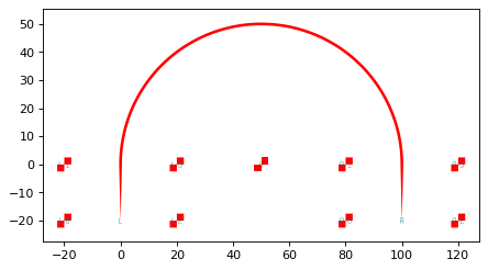
A first device

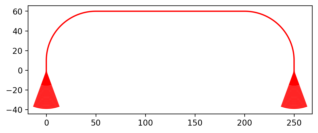
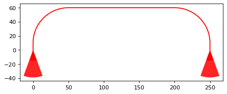
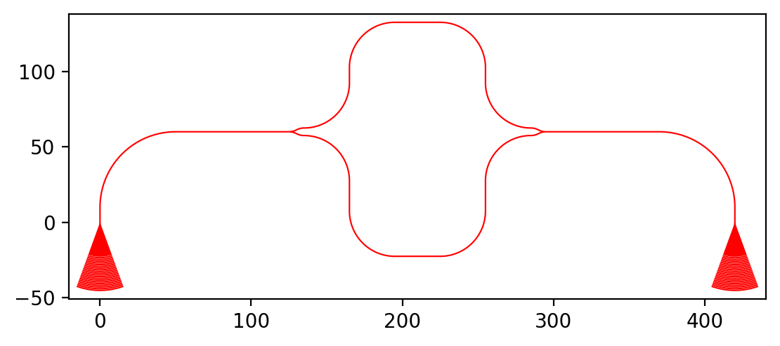
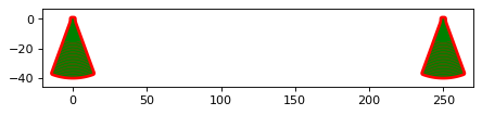
Our first device is going to be two grating couplers connected via a waveguide. This will be really simple

import numpy as np
from math import pi
from gdshelpers.geometry.chip import Cell
from gdshelpers.parts.waveguide import Waveguide
from gdshelpers.parts.coupler import GratingCoupler

coupler_params = {
    'width': 1.3,
    'full_opening_angle': np.deg2rad(40),
    'grating_period': 1.155,
    'grating_ff': 0.85,
    'n_gratings': 20,
    'taper_length': 16.
}

left_coupler = GratingCoupler.make_traditional_coupler(origin=(0, 0), **coupler_params)
wg = Waveguide.make_at_port(port=left_coupler.port)
wg.add_straight_segment(length=10)
wg.add_bend(angle=-pi / 2, radius=50)
wg.add_straight_segment(length=150)
wg.add_bend(angle=-pi / 2, radius=50)
wg.add_straight_segment(length=10)
right_coupler = GratingCoupler.make_traditional_coupler_at_port(port=wg.current_port, **coupler_params)

cell = Cell('SIMPLE_DEVICE')
cell.add_to_layer(1, left_coupler, wg, right_coupler)
cell.show()
# cell.save('chip.gds')

(Source code, png, hires.png, pdf)

Let’s go through that step by step:

The imports

The first paragraph contains import statements. These tell python which packages it should now in this program. While the import statement just imports the whole package path, the from ... import ... statement imports an object to the local namespace. So instead of writing math.pi all the time, from math import pi allows us to just use pi since Python now knows where the pi object came from. Several modules are listed here:

• math which is part of the Python standard library and also contains stuff such as sin() etc.
• gdshelpers which is what this tutorial is primarily about.

The part objects

We use two parts here: gdshelpers.parts.coupler.GratingCoupler and gdshelpers.parts.waveguide.Waveguide follow the links to get more information on them. When you look again at the source code creating the parts, you will see a Port mentioned. This port is just a construct designed to help the user. It bundles three properties inherent to any waveguide:

• Position
• Angle
• Width of the waveguide/port

All parts can also be placed by hand without the usage of ports – but its much simpler to use them.

Output to GDS

We previously created our part objects (left_coupler, wg and right_coupler) but we need to add it to our GDS file somehow. A bit of background might be in order here: GDS files are really really old file formats. They have quite a lot of restrictions – the most serious of them is the limit of 200 points per line or polygon. The device we have just created has definitely more points, so it has to be sliced or ‘fractured’. But fear not, the gdshelpers will take care of that for you. One of the nicer features of GDS files is their concept of CELLs. A layout can have several cells, each cell can contain other cells. If the cells are identical, GDS will just use a reference to the cell, saving time and space. In the code above we created a cell SIMPLE_DEVICE and added it to our layout. If you are a Cadence EDA user, you might be a bit confused now. This is because in Cadence most users just use one big cell for painting. But Cadence EDA actually supports cells.

Finish the chip

Now, lets run that code by clicking on that green play icon in the top toolbar. You will see a new window showing you what you just designed. Additionally, a new file called chip.gds appears in your project folder. The is the GDS file we wanted to create. You can open it in KLayout now.

Exercises

Please also take your time to extend your chip according to the images. You can see one possible solution by clicking on Source code above the image.

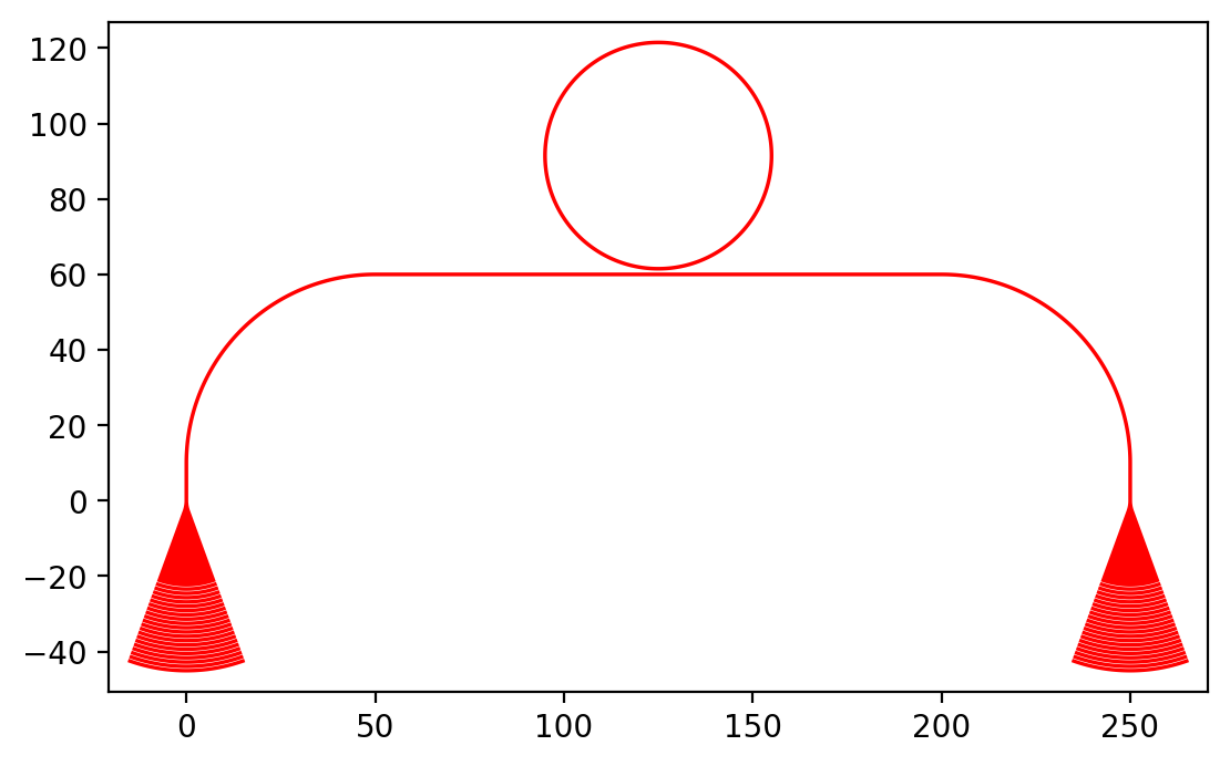
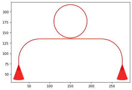
Insert a resonator

Use gdshelpers.parts.resonator.RingResonator to add a ring resonator to your design.

(Source code, png, hires.png, pdf)

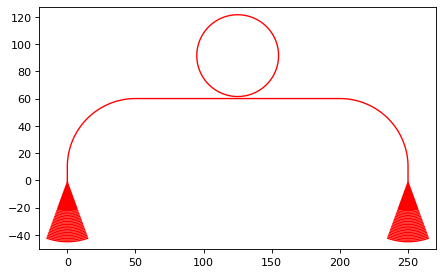
You might also want to play around with the possible extra parameters. Try race_length, res_wg_width. What happens if the gap is negative?

Insert a Mach-Zehnder interferometer

You can also easily insert a Mach-Zehnder interferometer, since it is already included in the parts. Try out the gdshelpers.parts.interferometer.MachZehnderInterferometer class.

(Source code, png, hires.png, pdf)

Note, how the interferometer is basically just composed of the parts we used before, except the Y-splitter. This part will be covered in the next device. For now, remember that if you ever plan to create your own part - MachZehnderInterferometer is a good place to start looking into the inner workings of gdshelpers.

Simple Drawing

While in the beginning it might be enough to use the included parts, you will quickly need to design your own parts and geometries. Remember that you will be using Shapely to generate your polygons. The only magic will be done internally when converting to gdsCAD.

Simple polygons

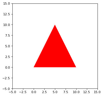
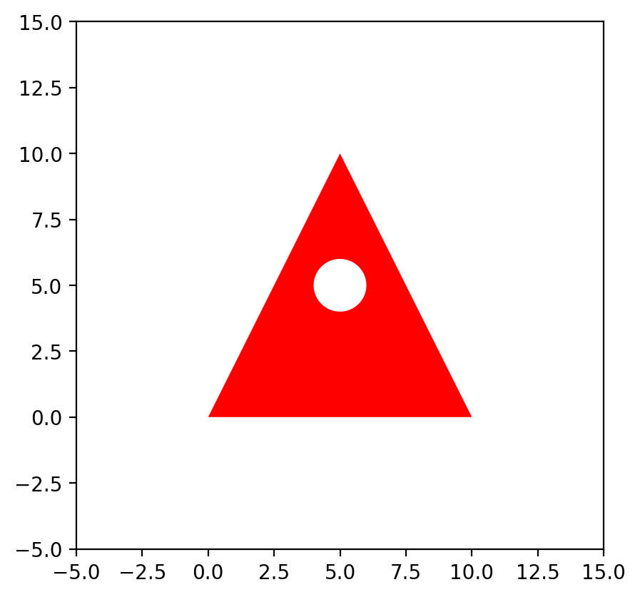
Let’s start with the most simple polygon one could think of - a triangle! Let the corners be at (0, 0), (10, 0) and (5, 10):

from gdshelpers.geometry.chip import Cell

from shapely.geometry import Polygon

outer_corners = [(0, 0), (10, 0), (5, 10)]
polygon = Polygon(outer_corners)

cell = Cell('POLYGON')
cell.add_to_layer(1, polygon)
cell.show()

(Source code, png, hires.png, pdf)

That’s simple, right? We import the Polygon from shapely.geometry just as we did with pi in the previous example. A Shapely polygon always has a outer hull and optional holes - which we did not use here.

You can easily build more complex polygons. But make sure, your outer lines do not cross because such polygons are not valid. One simple trick to clean such a invalid polygon is the obj.buffer(0) command. In this case, a self-intersecting polygon such as the classic “bowtie” will be split into two polygons. More recent versions of gdshelpers will try to produce an acceptable output even if the polygon is invalid. You will however still see an error message and it is strongly advised to fix up your code.

Generating a circle

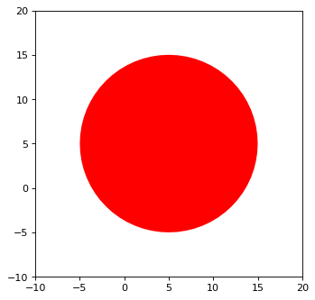
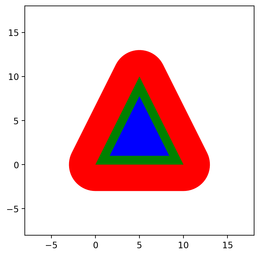
There is a neat trick to generate filled circles: A filled circle is nothing more than a Point, which has been “blown up” in all directions. It turns out that there all Shapely objects have a buffer() method. So we could increase the size of our triangle:

polygon = Polygon(outer_corners)
polygon_inflated = polygon.buffer(3.)
polygon_deflated = polygon.buffer(-1.)

(Source code, png, hires.png, pdf)

Naturally, this also works for Points:

point = Point(5, 5)
point_inflated = point.buffer(1.)

(Source code, png, hires.png, pdf)

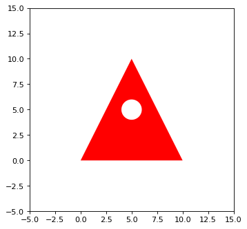
Boolean operations

Shapely includes a lot of boolean operations like a.difference(b), a.intersection(b), a.symmetric_difference(b) as well as a.union(b). The names should be self-explanatory, right? So let’s cut a hole into our triangle:

from shapely.geometry import Polygon, Point
from gdshelpers.geometry.chip import Cell

outer_corners = [(0, 0), (10, 0), (5, 10)]
polygon = Polygon(outer_corners)

point = Point(5, 5)
point_inflated = point.buffer(1)

cut_polygon = polygon.difference(point_inflated)

cell = Cell('POLYGON')
cell.add_to_layer(1, cut_polygon)
cell.show()

(Source code, png, hires.png, pdf)

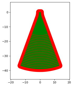
Using parts for polygon operation

Ok, so for now we used a Shapely object and its methods for polygon manipulation. Naturally, you can also use parts. When you go back to Software design and intended usage you will see that all parts provide a get_shapely_object() function. So this function will return a Shapely object which you can manipulate further:

from math import pi
from gdshelpers.geometry.chip import Cell
from gdshelpers.parts.waveguide import Waveguide
from gdshelpers.parts.coupler import GratingCoupler
from gdshelpers.parts.resonator import RingResonator

coupler_params = {
    'width': 1.3,
    'full_opening_angle': np.deg2rad(40),
    'grating_period': 1.155,
    'grating_ff': 0.85,
    'n_gratings': 20,
    'taper_length': 16.
}

coupler = GratingCoupler.make_traditional_coupler(origin=(0, 0), **coupler_params)
coupler_shapely = coupler.get_shapely_object()

# Do the manipulation
buffered_coupler_shapely = coupler_shapely.buffer(2)

cell = Cell('CELL')
cell.add_to_layer(1, buffered_coupler_shapely)
cell.add_to_layer(2, coupler_shapely)
cell.show()

(Source code, png, hires.png, pdf)

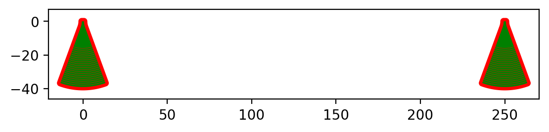
Using multiple parts and/or Shapely objects

Now, most of the times you will have to deal with multiple parts and maybe Shapely objects. Instead of calling get_shapely_object() for each part and building the common union of all parts, the gdshelpers.geometry.geometric_union() function provides a fast way of merging a list (or other kind of iterable) into one big Shapely container:

coupler_params = {
    'width': 1.3,
    'full_opening_angle': np.deg2rad(40),
    'grating_period': 1.155,
    'grating_ff': 0.85,
    'n_gratings': 20,
    'taper_length': 16.
}

coupler1 = GratingCoupler.make_traditional_coupler(origin=(0, 0), **coupler_params)
coupler2 = GratingCoupler.make_traditional_coupler(origin=(250, 0), **coupler_params)


both_coupler_shapely = geometric_union([coupler1, coupler2])
# Do the manipulation
buffered_both_coupler_shapely = coupler_shapely.buffer(2)

(Source code, png, hires.png, pdf)

Sweeping a parameter space

When you start designing your first chips you will probably have a simple chip design like the one introduced in A simple chip. Let’s say you already got a nice program which generates a cell with your device:

import numpy as np
from math import pi
from gdshelpers.geometry.chip import Cell
from gdshelpers.parts.waveguide import Waveguide
from gdshelpers.parts.coupler import GratingCoupler
from gdshelpers.parts.resonator import RingResonator

coupler_params = {
    'width': 1.3,
    'full_opening_angle': np.deg2rad(40),
    'grating_period': 1.155,
    'grating_ff': 0.85,
    'n_gratings': 20,
    'taper_length': 16.
}

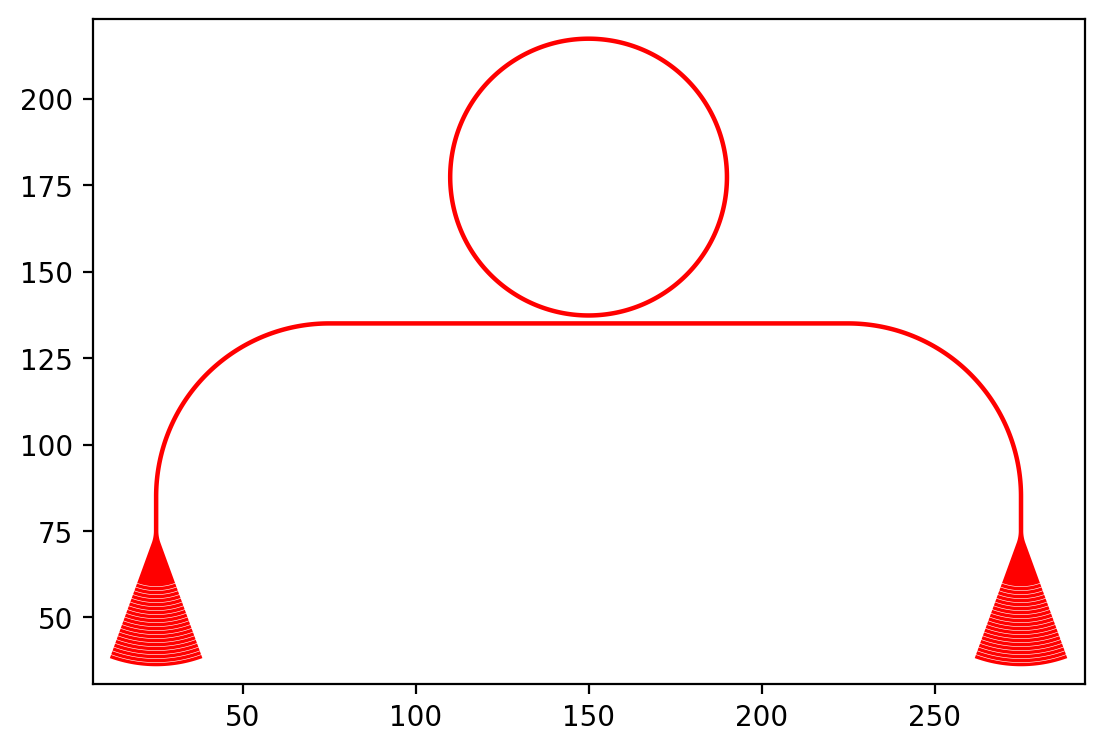
def generate_device_cell(resonator_radius, resonator_gap, origin=(25, 75)):
    left_coupler = GratingCoupler.make_traditional_coupler(origin, **coupler_params)
    wg1 = Waveguide.make_at_port(left_coupler.port)
    wg1.add_straight_segment(length=10)
    wg1.add_bend(-pi/2, radius=50)
    wg1.add_straight_segment(length=75)

    ring_res = RingResonator.make_at_port(wg1.current_port, gap=resonator_gap, radius=resonator_radius)

    wg2 = Waveguide.make_at_port(ring_res.port)
    wg2.add_straight_segment(length=75)
    wg2.add_bend(-pi/2, radius=50)
    wg2.add_straight_segment(length=10)
    right_coupler = GratingCoupler.make_traditional_coupler_at_port(wg2.current_port, **coupler_params)

    cell = Cell('SIMPLE_RES_DEVICE')
    cell.add_to_layer(1, left_coupler, wg1, ring_res, wg2, right_coupler)
    return cell

example_device = generate_device_cell(40., 1.)
example_device.show()

(Source code, png, hires.png, pdf)

Note, how the generate_device_cell creates one single gdsCAD cell per device. For now we just picked two random values for the resonator radius and the gap between the waveguides. Now, how do we sweep over several parameters and add them to those nice layouts with labels and a frame around it? You could create a new cell and add a reference to the device cells to it. 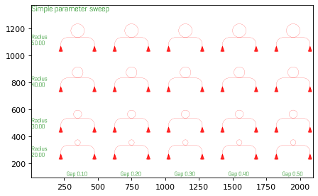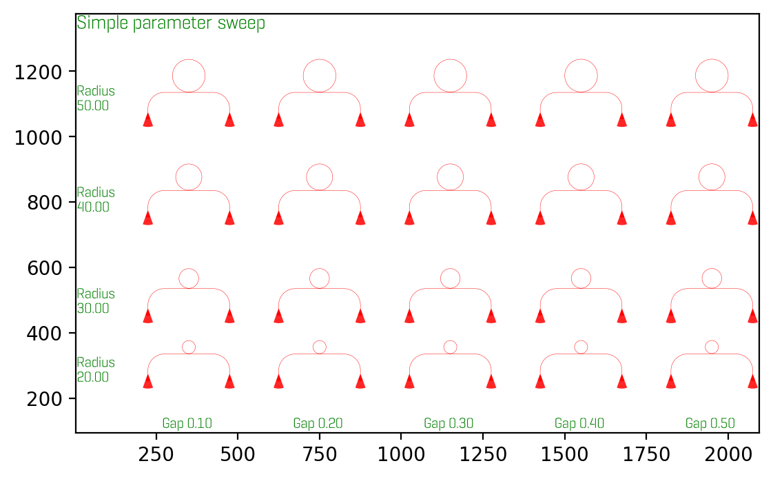While adding a cell reference in gdsCAD you can also specify transformations like translation and/or rotation. For now, we are just after a simple standard layout, so we can use the GridLayout included in gdshelpers:

layout = GridLayout(title='Simple parameter sweep')
radii = np.linspace(10, 20, 4)
gaps = np.linspace(0.1, 0.5, 5)

# Add column labels
layout.add_column_label_row(('Gap %0.2f' % gap for gap in gaps), row_label='')

for radius in radii:
    layout.begin_new_row('Radius\n%0.2f' % radius)
    for gap in gaps:
        layout.add_to_row(generate_device_cell(radius, gap))

layout_cell, mapping = layout.generate_layout()
layout_cell.show()

(Source code, png, hires.png, pdf)

By default GridLayout will place all devices on a regular grid as close as possible - while maintaining a minimum spacing and aligning to write fields. If your original cell was optimized to write fields (this one was not), your generated layout will also be within the write fields. To profit from this, assume your write field starts at (0, 0). This is valid, even if your electron beam write starts its write field at the top left structure. The frame of the layout will force a correct write field in this case. If you worked with older versions of gdshelper, you might have used TiledLayout which was the initial attempt on a device layout manager. Unfortunately, it proved to be unflexible. If you want to pack your devices as close as possible in the x-direction. Pass tight=True to the GridLayout constructor. Region layers can either be placed per cell, or per layout. The region layer behaviour can be changed with the region_layer_type and region_layer_on_labels parameters. Refere to the TiledLayout documentation for more details. Also note, that GridLayout.generate_layout() returns two values. We have only used the first value layout_cell. The value in mapping will tell you where each device was placed. To make use of this, you have to pass a unique id when calling add_to_row.

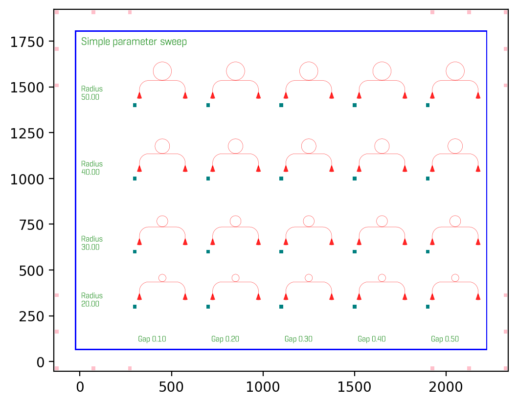
Generating electron beam lithography markers

When writing several layers with electron beam lithography, markers are needed to align these layers. There is a class in gdshelpers that will help you to generate these markers. Note that at the moment only square markers can be found in the library. However, other types of markers can easily be added by writing an own frame_generator and then using the same method. Here is one example how global and local markers can be added:

import numpy as np

from math import pi
from gdshelpers.geometry.chip import Cell
from gdshelpers.parts.waveguide import Waveguide
from gdshelpers.parts.coupler import GratingCoupler
from gdshelpers.parts.resonator import RingResonator
from gdshelpers.layout import GridLayout
from gdshelpers.parts.marker import SquareMarker
from gdshelpers.geometry.ebl_frame_generators import raith_marker_frame

coupler_params = {
    'width': 1.3,
    'full_opening_angle': np.deg2rad(40),
    'grating_period': 1.155,
    'grating_ff': 0.85,
    'n_gratings': 20,
    'taper_length': 16.
}

def generate_device_cell(resonator_radius, resonator_gap, origin=(25, 75)):
    left_coupler = GratingCoupler.make_traditional_coupler(origin, **coupler_params)
    wg1 = Waveguide.make_at_port(left_coupler.port)
    wg1.add_straight_segment(length=10)
    wg1.add_bend(-pi / 2, radius=50)
    wg1.add_straight_segment(length=75)

    ring_res = RingResonator.make_at_port(wg1.current_port, gap=resonator_gap, radius=resonator_radius)

    wg2 = Waveguide.make_at_port(ring_res.port)
    wg2.add_straight_segment(length=75)
    wg2.add_bend(-pi / 2, radius=50)
    wg2.add_straight_segment(length=10)
    right_coupler = GratingCoupler.make_traditional_coupler_at_port(wg2.current_port, **coupler_params)

    cell = Cell('SIMPLE_RES_DEVICE r={:.1f} g={:.1f}'.format(resonator_radius, resonator_gap))
    cell.add_to_layer(1, left_coupler, wg1, ring_res, wg2, right_coupler)
    cell.add_ebl_marker(layer=9, marker=SquareMarker(origin=(0, 0), size=20))
    return cell


layout = GridLayout(title='Simple parameter sweep', frame_layer=0, text_layer=2, region_layer_type=None)
radii = np.linspace(20, 50, 4)
gaps = np.linspace(0.1, 0.5, 5)

# Add column labels
layout.add_column_label_row(('Gap %0.2f' % gap for gap in gaps), row_label='')

for radius in radii:
    layout.begin_new_row('Radius\n%0.2f' % radius)
    for gap in gaps:
        layout.add_to_row(generate_device_cell(radius, gap))

layout_cell, mapping = layout.generate_layout()
layout_cell.add_frame(frame_layer=8, line_width=7)
layout_cell.add_ebl_frame(layer=10, frame_generator=raith_marker_frame, n=2)
layout_cell.show()

(Source code, png, hires.png, pdf)

First of all, we can add local EBL markers with add_ebl_marker and a defined position. Secondly, global markers are added with add_ebl_frame, and the number of markers per corner can be adjusted by changing the parameter n. In addition to the EBL markers, we added a frame around our structures with add_frame.

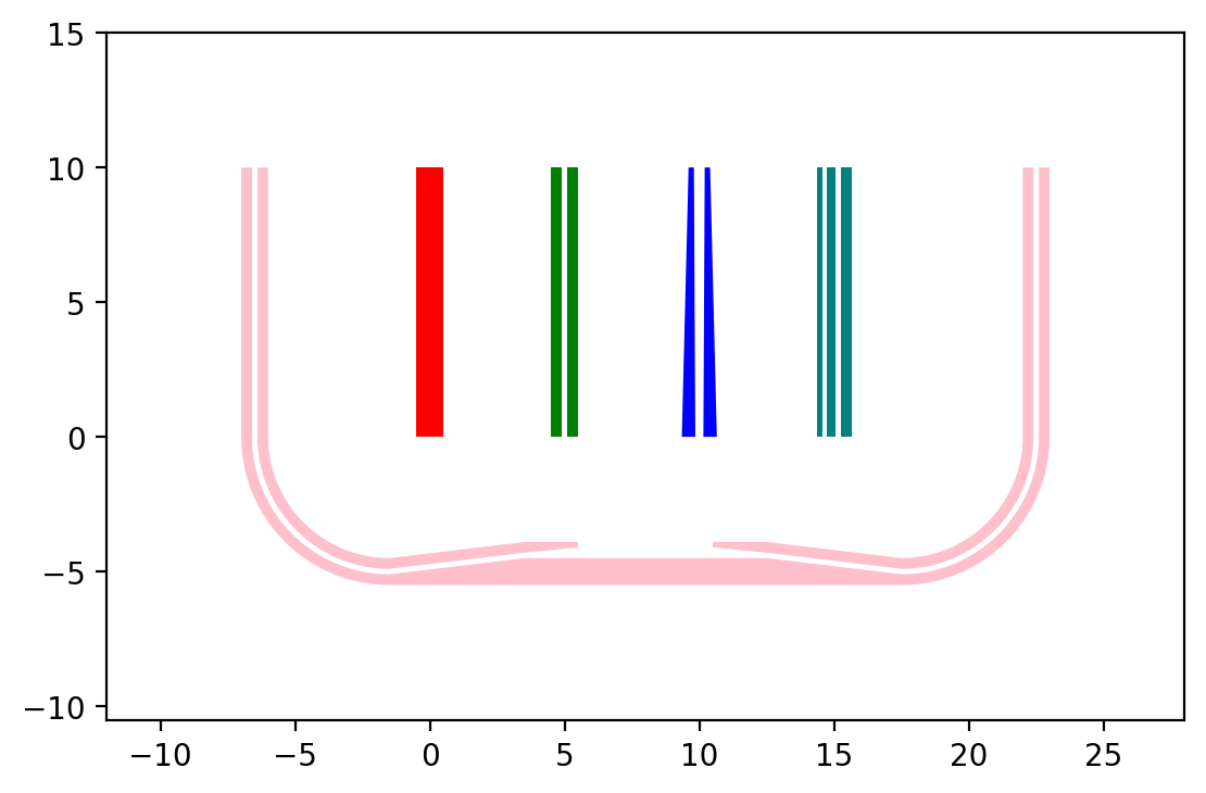
Slot waveguides and mode converters

So far, only strip waveguides have been used. However, gdshelpers includes also slot waveguides and strip-to-slot mode converters. Some examples are shown below:

import numpy as np

from gdshelpers.geometry.chip import Cell
from gdshelpers.parts.mode_converter import StripToSlotModeConverter
from gdshelpers.parts.waveguide import Waveguide
from gdshelpers.parts.port import Port

# waveguide 1: strip waveguide
wg_1 = Waveguide.make_at_port(Port(origin=(0, 0), angle=np.pi / 2, width=1))
wg_1.add_straight_segment(length=10)

# waveguide 2: slot waveguide
wg_2 = Waveguide.make_at_port(Port(origin=(5, 0), angle=np.pi / 2, width=[0.4, 0.2, 0.4]))
wg_2.add_straight_segment(length=10)

# waveguide 3: slot waveguide with tapering
wg_3 = Waveguide.make_at_port(Port(origin=(10, 0), angle=np.pi / 2, width=[0.5, 0.3, 0.5]))
wg_3.add_straight_segment(length=10, final_width=[0.2, 0.4, 0.2])

# waveguide 4: slot waveguide with three rails and two slots
wg_4 = Waveguide.make_at_port(Port(origin=(15, 0), angle=np.pi / 2, width=[0.2, 0.2, 0.3, 0.2, 0.4]))
wg_4.add_straight_segment(length=10)

# waveguide 5: slot waveguide with bends and strip to slot mode converter
wg_5_1 = Waveguide.make_at_port(Port(origin=(-6.5, 10), angle=-np.pi / 2, width=[0.4, 0.2, 0.4]))
wg_5_1.add_straight_segment(length=10)
wg_5_1.add_bend(angle=np.pi / 2, radius=5)
mc_1 = StripToSlotModeConverter.make_at_port(port=wg_5_1.current_port, taper_length=5, final_width=1,
                                             pre_taper_length=2, pre_taper_width=0.2)
wg_5_2 = Waveguide.make_at_port(port=mc_1.out_port)
wg_5_2.add_straight_segment(5)
mc_2 = StripToSlotModeConverter.make_at_port(port=wg_5_2.current_port, taper_length=5, final_width=[0.4, 0.2, 0.4],
                                             pre_taper_length=2, pre_taper_width=0.2)
wg_5_3 = Waveguide.make_at_port(port=mc_2.out_port)
wg_5_3.add_bend(angle=np.pi / 2, radius=5)
wg_5_3.add_straight_segment(length=10)

cell = Cell('Cell')
cell.add_to_layer(1, wg_1)  # red
cell.add_to_layer(2, wg_2)  # green
cell.add_to_layer(3, wg_3)  # blue
cell.add_to_layer(4, wg_4)  # jungle green
cell.add_to_layer(5, wg_5_1, mc_1, wg_5_2, mc_2, wg_5_3) # pink
cell.show()

(Source code, png, hires.png, pdf)

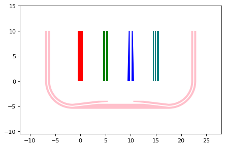
The routing is very similar to the routing of a strip waveguide, meaning that a port (origin, angle and width) has to be defined, and waveguides elements can be added from this port. The only difference is that the width of the waveguide is not given by a scalar, as shown in the case of waveguide 1, but by an array, usually with an odd number of elements. In this array, each element with an odd number denotes the width of a rail (waveguide 2), while each element with an even number denotes the width of the slot between two rails. As in the case of strip waveguides, one can make use of tapering (waveguide 3), bends (waveguide 5_1 and 5_3) and all other kinds of routing functions that are available in the Waveguide class.

Using the StripToSlotModeConverter class, strip to slot mode converters can added, which allow for a transition from a strip waveguide to a slot waveguide and vice versa. To create this element, five parameters have to be defined: The current port (origin, angle and width), the length of the taper, the final width and the width and length of the pre taper. If the current port width is a scalar and the final width is an array with three elements (two rails and one slot), a strip to slot mode converter is created. In the opposite case, a slot to strip mode converter is defined.

More advanced waveguide features

In the previous chapter, the waveguide part was already introduced and commonly used. While you might already be satisfied with what you got there, there are still a lot more useful hidden features.

Chaining of add_ calls

You will find yourself often calling several successive add_ type methods which will use lots of source code space. Code such as this:

wg = Waveguide.make_at_port(left_coupler.port)
wg.add_straight_segment(length=10)
wg.add_bend(-pi/2, radius=50)
wg.add_straight_segment(length=150)
wg.add_bend(-pi/2, radius=50)
wg.add_straight_segment(length=10)

Can be rewritten by chaining the construction calls:

wg = Waveguide.make_at_port(left_coupler.port)
wg.add_straight_segment(length=10).add_bend(-pi/2, radius=50)
wg.add_straight_segment(length=150).add_bend(-pi/2, radius=50)
wg.add_straight_segment(length=10)

This works, since all add_ type methods return the modified waveguide object itself again, which you can then call just as you do with wg..

Length measurements

Sometimes it is important to get the length of a Waveguide. Simply query .length to get the length of a waveguide. This even works for parameterized paths, but naturally it will only be a numerical approximation.

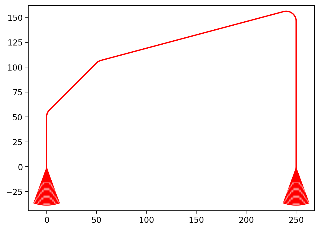
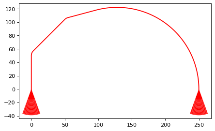
Automatic routing

Lot’s of times you will want to connect two points, but you always have to calculate the distance and factor in the bending radius etc. Since this is boring work and prone to error, a lot of useful routing functions are include in the Waveguide class. Available functions are:

• Waveguide.add_bezier_to() and Waveguide.add_bezier_to_port()
• Waveguide.add_route_single_circle_to() and Waveguide.add_route_single_circle_to_port()
• Waveguide.add_straight_segment_to_intersection()
• Waveguide.add_straight_segment_until_level_of_port()
• Waveguide.add_straight_segment_until_x() and Waveguide.add_straight_segment_until_y()

It’s probably best explained by an example. But if your are interested you can also check out the Waveguide class documentation:

import numpy as np
from math import pi
from gdshelpers.geometry.chip import Cell
from gdshelpers.parts.waveguide import Waveguide
from gdshelpers.parts.coupler import GratingCoupler

coupler_params = {
    'width': 1.3,
    'full_opening_angle': np.deg2rad(40),
    'grating_period': 1.155,
    'grating_ff': 0.85,
    'n_gratings': 20,
    'taper_length': 16.
}

left_coupler = GratingCoupler.make_traditional_coupler((0,0), **coupler_params)
right_coupler = GratingCoupler.make_traditional_coupler((250,0), **coupler_params)

wg = Waveguide.make_at_port(left_coupler.port)
wg.add_straight_segment_until_y(50)
wg.add_bend(np.deg2rad(-45), 10)
wg.add_straight_segment_until_x(50)
wg.add_bend(np.deg2rad(-30), 10)
wg.add_route_single_circle_to_port(right_coupler.port, 10)

cell = Cell('SIMPLE_DEVICE')
cell.add_to_layer(1, left_coupler, wg, right_coupler)
cell.show()

(Source code, png, hires.png, pdf)

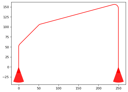
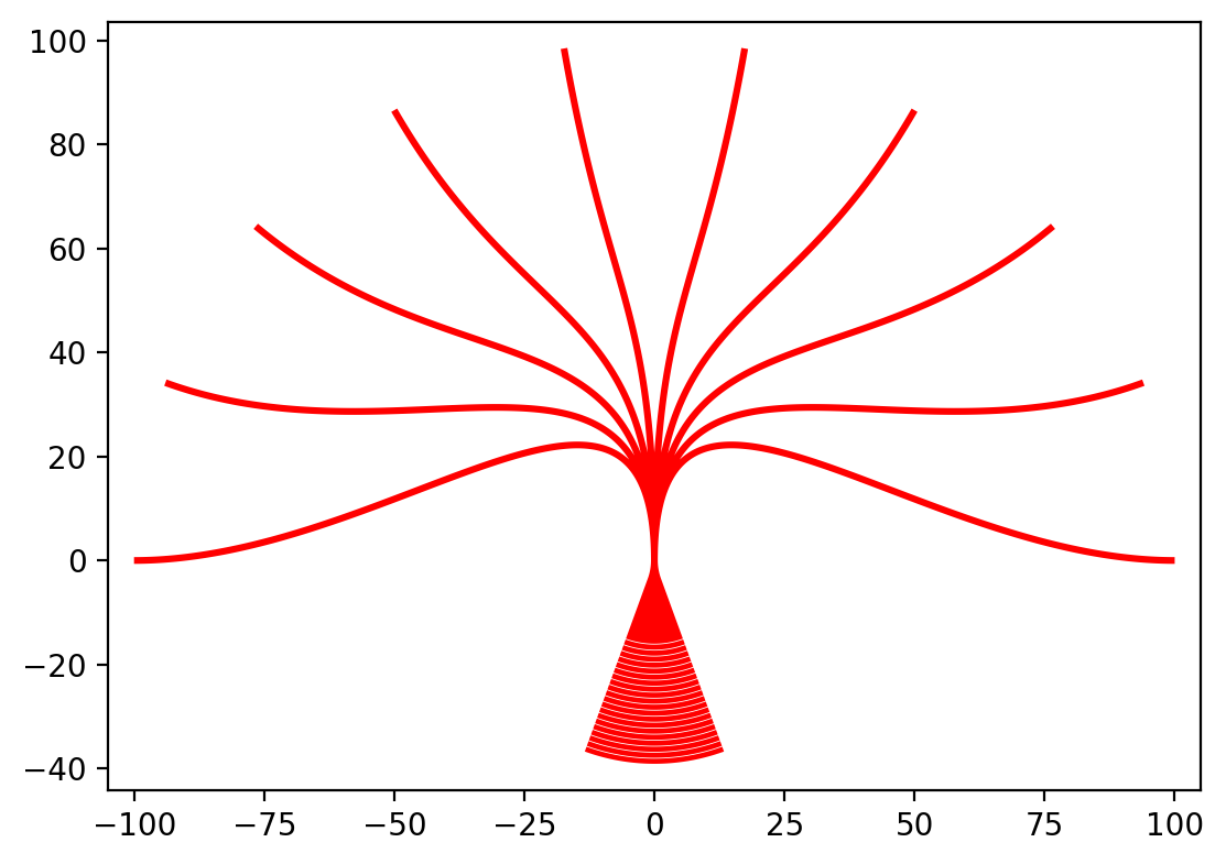
One other useful feature of Waveguide.add_route_single_circle_to() is that it will attempt to use the biggest possible bend radius if no maximal bend radius is specified:

wg.add_route_single_circle_to_port(right_coupler.port)

(Source code, png, hires.png, pdf)

If the maximum bend radius is set to zero, you will get a sharp edge.

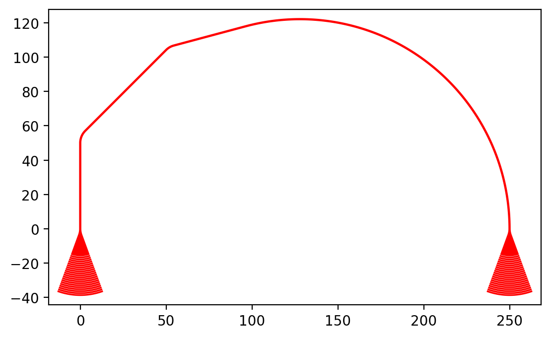
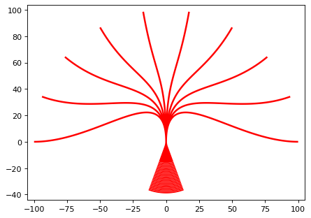
What we have omitted until now, is Bézier curve routing. This routing is special in the sense that it will give you smooth lines only. There will basically be no straight lines or circles. An example:

import numpy as np
from math import pi
from gdshelpers.geometry.chip import Cell
from gdshelpers.parts.waveguide import Waveguide
from gdshelpers.parts.coupler import GratingCoupler


coupler_params = {
    'width': 1.3,
    'full_opening_angle': np.deg2rad(40),
    'grating_period': 1.155,
    'grating_ff': 0.85,
    'n_gratings': 20,
    'taper_length': 16.
}

coupler = GratingCoupler.make_traditional_coupler((0,0), **coupler_params)
wgs = list()
for angle in np.linspace(-np.pi/2, np.pi/2, 10):
    # Calculate the target port
    # We do this by changing the angle of the coupler port and calculating a
    # longitudinal offset. Since the port then points outwards, we invert its direction.
    target_port = coupler.port.rotated(angle).longitudinal_offset(100).inverted_direction

    wg = Waveguide.make_at_port(coupler.port)
    wg.add_bezier_to_port(target_port, bend_strength=50)
    wgs.append(wg)

cell = Cell('SIMPLE_DEVICE')
cell.add_to_layer(1, coupler)
cell.add_to_layer(1, *wgs)
cell.show()

(Source code, png, hires.png, pdf)

Notice the bend_strength parameter of Waveguide.add_bezier_to_port(). The heigher the parameter, the smoother the connecting lines will be. But take care: For big values the Bézier curve might intersect with itself which will give you an error. In short, Bézier curves can be very useful to connect to non-trivial points - but they might give you errors on self intersection and are generally quite slow to calculate.

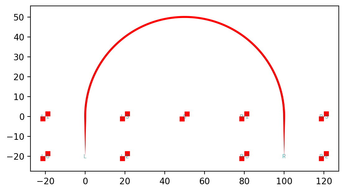
Interfacing 3D-hybrid structures

For interfacing integrated planar circuitry with 3D-hybrid structures, tapers need to be included into the design. In the vicinity of each taper alignment markers need to be included as well, allowing determination of the taper positions using computer vision.

This can simply be done by using the method Cell.add_dlw_taper_at_port(). The first parameter defines the name of the taper within the cell. In order to assure unique names, the complete name of the Cell includes the names of the surrounding cells separated by dots (but not the topmost cell, as there’s anyway just one). E.g. in the following example, the name of the tapers are defined as A0.L and A0.R. For each taper four alignment markers are generated automatically around the taper. Each marker name is composed by the name of the taper and an postfix -X, where X is a number from 0-3. The exact naming is shown in the layout on the comments layer.

(Source code, png, hires.png, pdf)

Besides automatically generated markers, the user can also directly add markers to the layout using add_dlw_marker() as shown in the example. This is on the one side handy for adding reference markers on the topmost level of the design, allowing for simple names (The marker in the example is just called “0”, as it’s on the topmost level, there are no cell names as prefixes). On the other hand, manual adding of the tapers is required, if the standard locations of the markers are already used by other elements in the design. By passing with_tapers=False as an parameter to Cell.add_dlw_taper_at_port(), automatic generation of the markers can be suppressed and the user is required to place the markers.

Fonts

It is always a good idea to label your designs extensively. Naturally, text is also supported in gdshelpers.

Gdshelpers supports its own font, using pure Shapely objects.

(Source code, png, hires.png, pdf)

Writing text

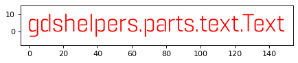
You have heard a lot about different text and label types now. Let’s get our hands dirty. The gdshelpers.parts.text.Text class behaves like any other part you already now. Typically you pass at least three options: origin, the text height and the actual text:

from gdshelpers.parts.text import Text
text = Text([0, 0], 10, 'gdshelpers.parts.text.Text')

(Source code, png, hires.png, pdf)

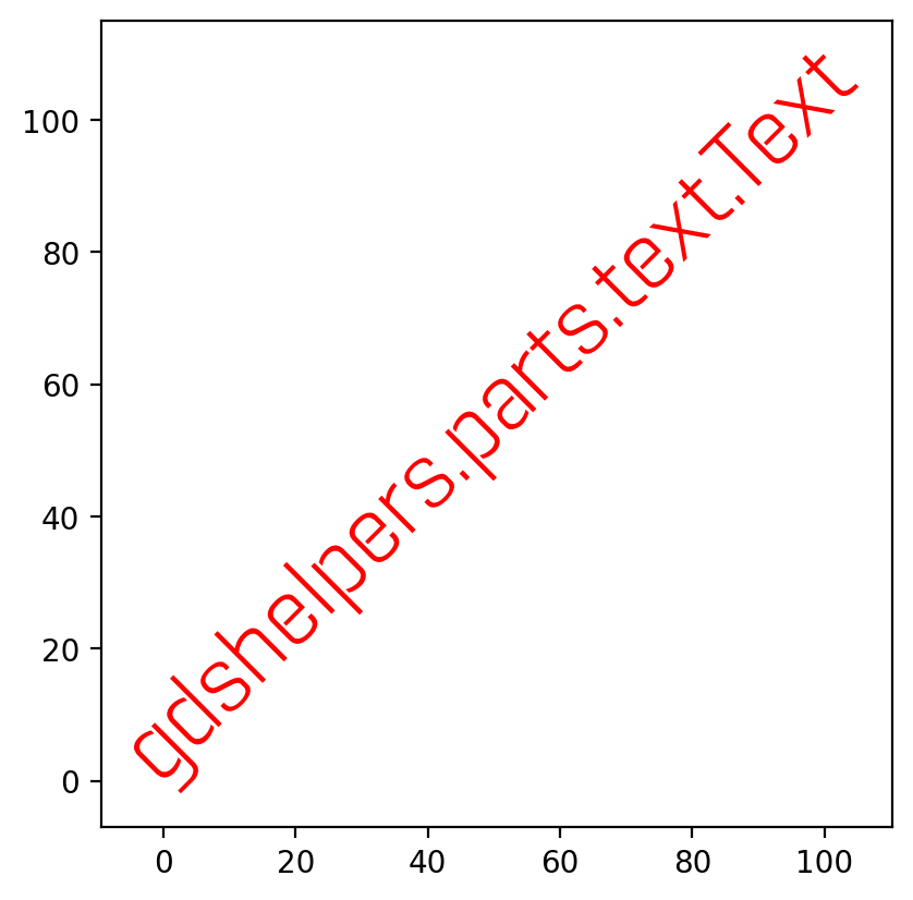
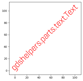
You can additionally specify an angle:

text = Text([0, 0], 10, 'gdshelpers.parts.text.Text', angle=np.pi/4)

(Source code, png, hires.png, pdf)

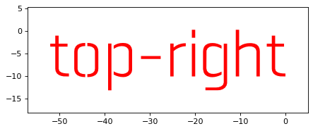
Another handy option is the alignment option. It lets you specify the alignment of the text. Alignment can be set independently for the x- and y-axis. Valid options are left, center, right for the x axis and bottom, center, top for the y-axis. So right-top will center the text to the upper right corner:

text = Text([0, 0], 10, 'top-right', alignment='right-top')

(Source code, png, hires.png, pdf)

Note

You can also write multiple lines at the same time! Simply use the \n character:

text = Text([0, 0], 10, 'The quick brown fox\njumps over the lazy dog\n1234567890',
            alignment='center-top')

(Source code, png, hires.png, pdf)

Final words

We now reached the end of this tutorial. In the next chapters we’ll focus on the growling list of parts implemented in this library.